Multivariable Calculus – Integral & Theorem Cheat Sheet
Conventions.
- In 2D: $\mathbf{F}=\langle M,N\rangle$. In 3D: $\mathbf{F}=\langle P,Q,R\rangle$.
- A smooth curve $C$ is parameterized by $\mathbf{r}(t)$, $a\le t\le b$.
- A smooth surface $S$ is parameterized by $\mathbf{r}(u,v)$ on a domain $D_{uv}$.
- Unit normal $\mathbf{n}$ is chosen by orientation (right-hand rule when paired with boundary orientation).
1) Line Integrals
Scalar line integral (with respect to arc length)
$$ \int_C f,ds ;=; \int_a^b f(\mathbf{r}(t)),|\mathbf{r}‘(t)|,dt. $$
Vector line integral (work)
$$ W=\int_C \mathbf{F}\cdot d\mathbf{r} ;=; \int_a^b \mathbf{F}(\mathbf{r}(t))\cdot \mathbf{r}‘(t),dt. $$
Work/energy interpretation: moving a particle through a force field $\mathbf{F}$ along $C$.
“Is $\mathbf{F}$ conservative?” (in a simply connected open set)
- Equivalent tests:
- $\displaystyle \oint_C \mathbf{F}\cdot d\mathbf{r}=0$ for every closed $C$.
- Path independence: $\int_{C_1}\mathbf{F}\cdot d\mathbf{r}=\int_{C_2}\mathbf{F}\cdot d\mathbf{r}$ for any two paths with same endpoints.
- There exists potential $f$ with $\mathbf{F}=\nabla f$.
- In 2D: $N_x=M_y$. In 3D: $\nabla\times \mathbf{F}=\mathbf{0}$.
Finding $f$ when conservative (2D): Integrate $M=\partial f/\partial x$ in $x$, then determine the “constant in $x$” via $N=\partial f/\partial y$.
2) Green’s Theorem (2D)
Let $C$ be positively oriented, piecewise smooth, simple closed curve bounding region $D$ and $M,N$ have continuous partials on an open set containing $D$.
Circulation form
$$ \oint_C M,dx+N,dy ;=; \iint_D \left(N_x - M_y\right),dA. $$
Flux / normal form
$$ \oint_C \mathbf{F}\cdot \mathbf{n},ds ;=; \oint_C (-N),dx + M,dy ;=; \iint_D \left(M_x + N_y\right),dA ;=; \iint_D \nabla\cdot\mathbf{F},dA. $$
Area corollaries
$$ \text{Area}(D)=\frac12\oint_C (x,dy - y,dx) ;=;\oint_C x,dy ;=; -\oint_C y,dx \quad (\text{choose any one}). $$
3) Surface Integrals
Scalar surface integral
Given $\mathbf{r}(u,v)$ on $D_{uv}$,
$$\iint_S f,dS ;=; \iint_{D_{uv}} f(\mathbf{r}(u,v)),|\mathbf{r}_u\times \mathbf{r}_v|,du,dv.$$
For a graph $z=g(x,y)$:
$$ dS = \sqrt{1+g_x^2+g_y^2},dx,dy. $$
Flux of a vector field across a surface
$$ \iint_S \mathbf{F}\cdot \mathbf{n},dS ;=; \iint_{D_{uv}} \mathbf{F}(\mathbf{r}(u,v))\cdot\left(\mathbf{r}_u\times \mathbf{r}_v\right),du,dv. $$
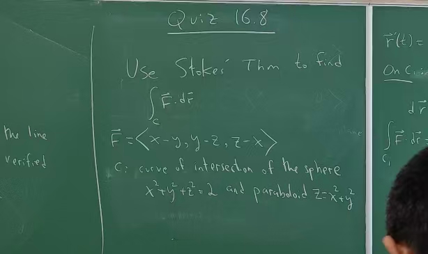
4) Stokes’ Theorem (3D)
Let $S$ be an oriented smooth surface with boundary curve $C=\partial S$ (positively oriented by the right-hand rule). If $\mathbf{F}$ has continuous partials,
$$ \oint_C \mathbf{F}\cdot d\mathbf{r} ;=; \iint_S (\nabla\times\mathbf{F})\cdot \mathbf{n},dS. $$
5) Divergence Theorem (Gauss)
Let $E$ be a solid region with boundary surface $S=\partial E$ oriented outward, and $\mathbf{F}$ have continuous partials:
$$ \iint_S \mathbf{F}\cdot \mathbf{n},dS ;=; \iiint_E \nabla\cdot\mathbf{F},dV. $$
6) Double & Triple Integrals
Double integral (Cartesian)
$$ \iint_D f(x,y),dA ;=; \int_{x=a}^b\int_{y=g_1(x)}^{g_2(x)} f(x,y),dy,dx \quad \text{or} \quad \int_{y=c}^d\int_{x=h_1(y)}^{h_2(y)} f(x,y),dx,dy. $$
Double integral (polar)
Use $x=r\cos\theta,;y=r\sin\theta,; dA = r,dr,d\theta$:
$$ \iint_D f(x,y),dA ;=; \int_{\theta=\alpha}^{\beta}\int_{r=r_1(\theta)}^{r_2(\theta)} f!\big(r\cos\theta, r\sin\theta\big); r,dr,d\theta. $$
Triple integral (Cartesian)
$$ \iiint_E f(x,y,z),dV ;=; \int!!\int!!\int f(x,y,z),dz,dy,dx \quad (\text{order to fit }E). $$
Triple integral (cylindrical)
Use $x=r\cos\theta,;y=r\sin\theta,;z=z,; dV=r,dr,d\theta,dz$:
$$ \iiint_E f,dV = \int_{\theta=\alpha}^{\beta}\int_{r=r_1(\theta)}^{r_2(\theta)}\int_{z=z_1(r,\theta)}^{z_2(r,\theta)} f(r\cos\theta,r\sin\theta,z); r,dz,dr,d\theta. $$
Triple integral (spherical)
Use $x=\rho\sin\phi\cos\theta,; y=\rho\sin\phi\sin\theta,; z=\rho\cos\phi,; dV=\rho^2\sin\phi,d\rho,d\phi,d\theta$:
$$ \iiint_E f,dV = \int_{\theta=\alpha}^{\beta}\int_{\phi=\phi_1(\theta)}^{\phi_2(\theta)}\int_{\rho=\rho_1(\phi,\theta)}^{\rho_2(\phi,\theta)} f(\rho,\phi,\theta); \rho^2\sin\phi, d\rho, d\phi, d\theta. $$
7) Change of Variables (Jacobian)
In 2D
If $(x,y)=(x(u,v),y(u,v))$ is one-to-one with nonzero Jacobian
$$ J=\frac{\partial(x,y)}{\partial(u,v)}= \begin{vmatrix} x_u & x_v\ y_u & y_v \end{vmatrix}, $$
then
$$ \iint_D f(x,y),dx,dy = \iint_{D^*} f\big(x(u,v),y(u,v)\big); \left|J\right|,du,dv. $$
In 3D
Similarly with $(x,y,z)=(x(u,v,w),y(u,v,w),z(u,v,w))$ and
$$ J=\frac{\partial(x,y,z)}{\partial(u,v,w)}= \det \begin{bmatrix} x_u & x_v & x_w\ y_u & y_v & y_w\ z_u & z_v & z_w \end{bmatrix}. $$
8) Curl and Divergence (Cartesian)
$$ \nabla\times\mathbf{F}=\begin{vmatrix} \mathbf{i} & \mathbf{j} & \mathbf{k}\ \partial_x & \partial_y & \partial_z\ P & Q & R \end{vmatrix} = \langle R_y-Q_z,; P_z-R_x,; Q_x-P_y\rangle. $$
$$ \nabla\cdot\mathbf{F} = P_x + Q_y + R_z. $$
Vector identities: $\nabla\times(\nabla f)=\mathbf{0}$, $\nabla\cdot(\nabla\times\mathbf{F})=0$.
9) Second Derivative Test (2D)
Let $f_x=f_y=0$ at $(a,b)$. Define
$$ D=f_{xx}(a,b),f_{yy}(a,b)-\big(f_{xy}(a,b)\big)^2. $$
- If $D>0$ and $f_{xx}(a,b)>0$: local minimum.
- If $D>0$ and $f_{xx}(a,b)<0$: local maximum.
- If $D<0$: saddle.
- If $D=0$: test inconclusive.
10) Lagrange Multipliers
One constraint $g(x,y,z)=c$:
Solve
$$ \nabla f=\lambda \nabla g,\qquad g(x,y,z)=c. $$
Two constraints $g(x,y,z)=c,; h(x,y,z)=k$:
$$ \nabla f=\lambda \nabla g+\mu \nabla h,\quad g=c,\quad h=k. $$
11) Flux (quick references)
- Across a plane curve $C$ (Green’s normal form):
$\displaystyle \oint_C \mathbf{F}\cdot \mathbf{n},ds = \oint_C (M,dy - N,dx) = \iint_D \nabla\cdot\mathbf{F},dA$. - Across a surface $S$:
$\displaystyle \iint_S \mathbf{F}\cdot \mathbf{n},dS=\iint_{D_{uv}}\mathbf{F}(\mathbf{r}(u,v))\cdot(\mathbf{r}_u\times\mathbf{r}_v),du,dv$. - Closed surface $S=\partial E$ (Divergence Thm):
$\displaystyle \iint_S \mathbf{F}\cdot \mathbf{n},dS=\iiint_E \nabla\cdot\mathbf{F},dV.$
12) Common Regional Setups (quick memory)
- Disk/annulus: use polar $(r,\theta)$, $dA=r,dr,d\theta$.
- Cylinder-like regions: use cylindrical $(r,\theta,z)$, $dV=r,dr,d\theta,dz$.
- Spheres/balls/cones: use spherical $(\rho,\phi,\theta)$, $dV=\rho^2\sin\phi,d\rho,d\phi,d\theta$.
Update on Aug 26th: This blog is written on Aug 14th, when i’m taking the exam at 12 a.m. And the $Latex$ display is failed, ChatGPT can’t fix that, quite disappointed. And finally i fixed it:)